Everything You Should Know About Return Loss Measurements Using a Directional Coupler
Contents
- 1. Introduction
- 2. Theory
- 3. Measuring reflection with a directional coupler
- 4. Applications
- 5. Conclusions
1. Introduction
Return loss is an important parameters of any RF (Radio Frequency) device. It is a measure of the amount of power reflected at a port. From it, impedance levels can be calculated and amplitude variations in transmission lines predicted. For one port devices, it is the only existing scattering parameter.
Usually, return loss is measured using a directional coupler. Therefore, these devices are studied in this article as well, including the measurement setup which is typically used. Also, the treatment of measurements errors is mandatory. Since they can influence return loss measurements more than we may wish.
The articles ends with descriptions of several useful applications for return loss measurements.
2. Theory
In this part we begin by looking at the ratio of the reflected- and incident- wave at an RF port. Note that this is also equal to the definition of the Sxx parameter.
Next, the relationship between the reflection coefficient and impedance mismatch of a transmission line is explained. Then we connect return loss measurements to the impedance mismatch at the end of a transmission line.
The next step is to look at a phenomenon called the Voltage Standing Wave Ratio (VSWR). It turns out that VSWR is just another parameter that exists due to the impedance mismatch at the end of the transmission line.
2.1 Reflection Coefficient and Impedance Mismatch
An ideal transmission line propagates waves without loss along its line. It carries two types of waves: a voltage and a current wave. The characteristic impedance of the transmission line defines the ratio between the voltage and current waves. By applying boundary conditions it can be shown that any discontinuity in impedance along the line will cause some part of the wave to travel in its reversed direction. So, at an impedance mismatch a part of the wave gets reflected back.
The ratio of reflected and incident power is called the reflection coefficient Γ ("Gamma").
It helps to look at some extreme examples. The first one to consider is a wave that propagates along a transmission line with an open end (ZL equals infinity). When the wave reaches the end of the line, it will be reflected back completely (Γ = 1). The same is true for a shorted transmission line (ZL equals zero). In this case, Γ = -1. The minus sign indicates the fact that the phase of the reflected wave is inverted now. If, on the other hand, the transmission line is terminated with an impedance that matches exactly the impedance of the transmission line (Z0), then there will be no energy reflected back (Γ = 0).
There is a nice (old, but instructive) video on YouTube that explains these types of reflection phenomena using a mechanical system.
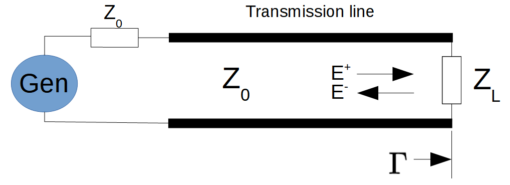
It turns out that there is a relation between the impedance mismatch and the reflection coefficient:
Γ = E- / E+
Γ = bi / ai = Sii
Γ = (ZL- Z0) / (ZL + Z0) (1)
This means that if we know Γ, we can calculate the impedance mismatch. Γ will be positive if ZL is larger then Z0 and negative when it is smaller. If we know Z0, the value of ZL can be calculate as well.
Note that Γ is also equivalent to the Sii parameter which is defined by the ratio between the reflected and incident power waves bi and ai. This equation is explained in more detail in the S-parameter article.
By rearranging equation (1) we can isolate ZL as :
ZL = [ (1 + Γ) / (1 - Γ) ] . Z0 (2)
You can verify that this equation gives you the right answers for the special cases looked at earlier in this paragraph. In general, ZL and Γ are complex numbers because they are vector quantities that incorporate phase information.
It is important to note that the characteristic impedance Z0 of a lossless transmission line has no reactance.
2.2 The Transformation from Impedance to Reflection Coefficient
In order to understand the relation (1) better we plotted Γ as a function of RL. We did so for several different magnitudes and for each magnitude, the phase was varied between -90 and +90 degrees. So, we changed the impedance ZL in steps from (pure) capacitive via the x-axis (no reactance) to (pure) inductive. Note that for all other intermediate steps the impedance has both a real and a reactive part. You will find these impedance plots depicted as half circles in Figure 2. There are no points with Re(ZL) <0 because we modelled passive loads only.
The bottom part of Figure 2 shows the corresponding values of the reflection coefficient Γ.
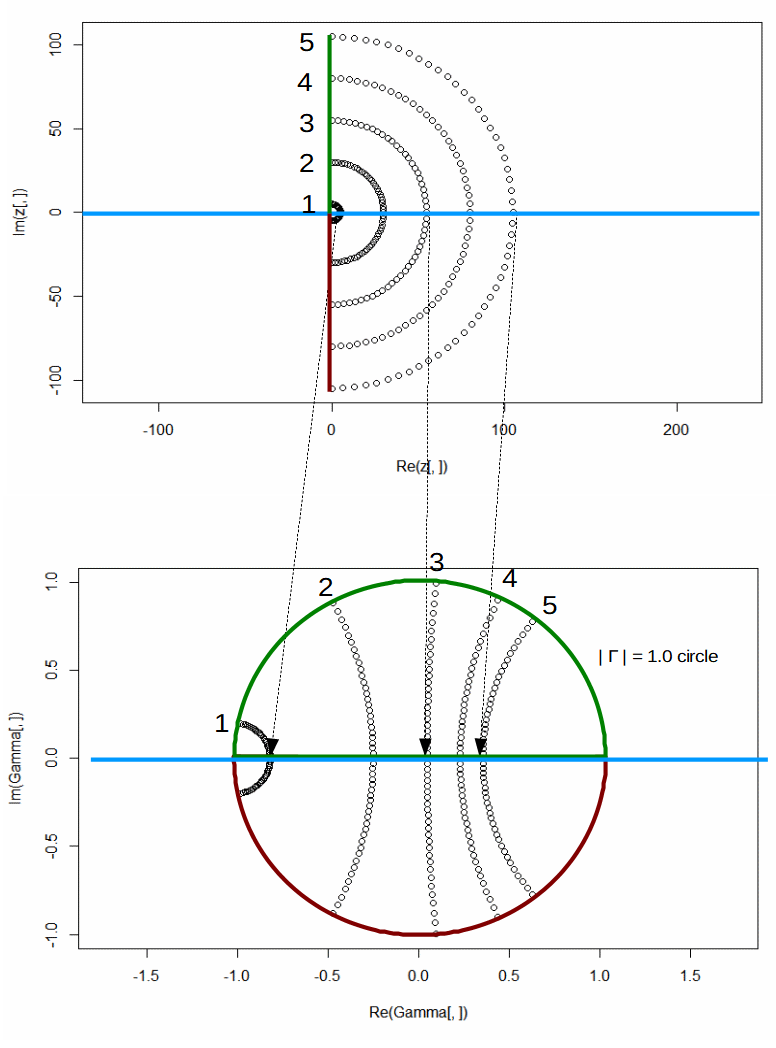
Now we can make the following observations
- A circles of |ZL| does not translate to a circle of constant magnitude for |Γ|. The phase shift of ZL has a profound influence on the magnitude of |Γ|.
- When the phase of ZL approaches + or -90 degrees, the corresponding point in the Γ plane moves to the |Γ| = 1 circle. This is expected because a pure reactive load cannot dissipate energy. So, all energy must be reflected back.
- Small values of |ZL| transform to Γ = -1 and for |ZL| approaching infinity we get at Γ = 1.
- All values of Γ lay within a circle with a radius of 1. This is because we limited RL to values with a non-negative real part.
- Impedance magnitudes that are bigger then |Z0| transform to the right side of the circle in the Γ plane and vice versa.
What we learn from all of this is that, in general, it is not possible to know ZL, unless we know both the magnitude and phase of Γ.
The plots also show that a reflection coefficient Γ of 0 is only possible at one point: where ZL = Z0. In our example Z0 equals 50 Ohms.
2.3 Calculating the Impedance from the Transmission Coefficient
If we know Γ, the impedance ZL can be calculated from (2). Remember that Γ is a complex number because it contains both magnitude and phase information. We can now plot RL using several values for both the magnitude and phase of Γ as input values. Figure 3 shows the result for three magnitudes of Γ ranging from 0.1 to 0.7, while varying the phase from 0 to 2π (radians) for each magnitude. The lower part of Figure 3 show the circles that are transformed by the relation (2) on the complex impedance plane.
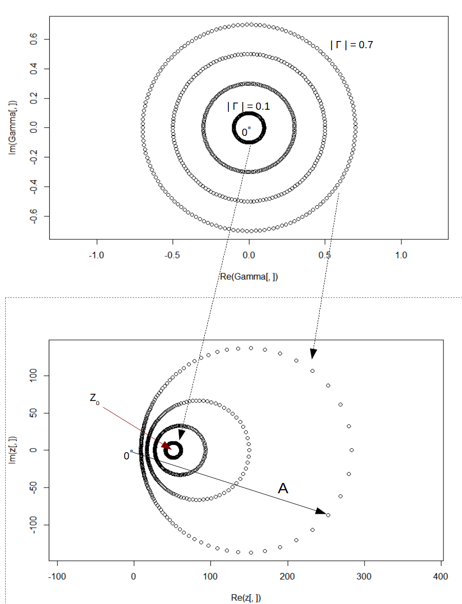
We can now make the following observations:
- Each circle of |Γ| equal to some value (<1), corresponds to a circle of possible impedances that lay in a circle too. If we wanted to know the magnitude and phase of the impedance as defined by vector A, laying at the circle that corresponds with |Γ| = 0.7 (in this example), then we must know the phase of Γ as well. If we don't, there is not much to say about the magnitude and phase of A.
- For very low values of |Γ| (approaching zero), the circle of possible impedances gets very small and converts around the impedance Z0. This also means that the smaller |Γ|, the less reactance is possessed by ZL.
- Not shown in the picture is the impedance circle for |Γ| = 1. This circle would lead to the plot of an extra circle in the impedance plot with a diameter of infinity. Using the same values along the axis, this would lead to only a small part of this circle being visible and it would render as a line segment along the imaginary axis. Similar to the relation |Γ| = 1 in Figure 2.
What we learn from this plot is that if we want to say something about the impedance ZL in general, we must know both the magnitude and phase of Γ. We can also, as a limited but valuable alternative, determine the mismatch of ZL to Z0 by looking at |Γ| only. The first approach involves using a Vector Network Analyzer, which measures magnitude and phase. The second method is the foundation underpinning return loss measurements with a Spectrum Analyzer, which measures magnitude only.
2.4 Impedance at the Near-End of the Transmission Line
Transmission lines that are matched to their characteristic impedance behave well. The observed impedance at the near end of the line is equal to ZL, independent of the length of the line or the frequency of operation. However, if ZL does not match the characteristic impedance Z0, this is not the case. In this case, the observed impedance will vary with the length of the transmission line and frequency.
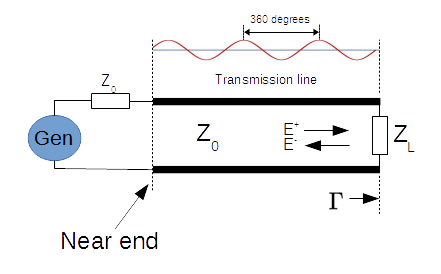
This is due to the reflected wave interfering with the incident wave, which alters the ratio between the voltage and current waves that define the impedance. This interference is dictated by phase differences, causing the waves to phase- add and subtract. And the phase of the waves changes with both the position at the line (d) and its wavelength (λ).
In this situation the impedance ZS at the near end of the line is calculated as (Figure 4)
ZS = [ (1 + Γe-4jd/λ) / (1 - Γe-4jd/λ) ] . Z0 (3)
This formula shows that the phase of Γ can be set to any value we like by changing the length (d) of the transmission line. Also, we know from Figure 3 that changing the phase of Γ has a strong effect on both the magnitude and phase of the perceived load.
This property is much used in RF design by using small transmission lines (e.g. 1/8 wavelength) with an open or closed termination (|Γ| = 1) called stubs, in filters and impedance matching circuits.
However, most of the times it is an annoyance if the performance of our system depends on line length or operating frequency. Therefore, in general, we try to minimize Γ by matching transmission lines to its characteristic impedance.
2.4.1 The Use of Port Extension
If we want to make an accurate measurement of Γ at the near end of the transmission line, in order to calculate RL, we get into serious trouble by the phase change created by the length of the line as explain in the previous section. An example of such a situation happens when we want to measure the return loss by using a Vector Network Analyzer (VNA). The problem is created when the length of the measurement cables is changed between the setup used during calibration and actual use. For example, when the DUT needs an adapter to connect to the test cable(s), which effectively extends the length of the cable.
This added length changes the relative phase at the plane of reference to any value between 0- and 360- degrees (Figure 4).
The situation is remedied by telling the VNA to compensate for the phase shift by specifying the travel time of the wave along the adapter. This way, the VNA virtually 'extends' the length of the measurement port. Hence the name port extension.
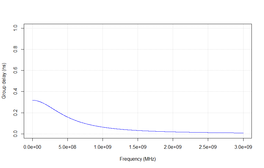
2.4.2 What is Group Delay?
Another topic worth looking at when we want to understand the influence of the length of the transmission line on a reflection measurement, is group delay. This parameter is defined as dΦ / dω, with Φ the phase and ω the frequency. It turns out that if you take the derivative of the phase with respect to frequency, you get an outcome with the unit time (radians / radians / second = second). This time represents the delay of the signal at the frequency ω.
In order to understand the nature of group delay, consider a wave that propagates through some medium. If we want to know how long it is traveling, we can look at the phase change (in radians) that the wave developed during its journey, and compare this phase change with some measure that tells us how long phase change takes. That is the frequency in radians / second. So, dΦ / dω is a measure for the time the wave has travelled. The group delay is defined as:
tg = -dΦ / dω
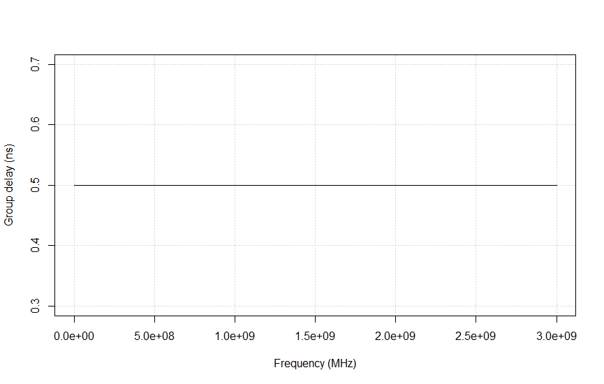
If a system dΦ / dω is equal to some constant (time) for every frequency, we denote that system as a linear phase system. Such systems delay every frequency by the same amount. A lossless transmission line has a linear phase response.
2.4.3 How to use Group Delay Information
Group delay can be used to set the Port Extension parameter. By measuring the group delay in a measurement setup after calibration, we get information about the extra time a wave needs to travel due to changes in the electrical line length, as discussed in paragraph 2.3.1. This travel time is determined by measuring the group delay and using it in the port extension procedure. Most VNAs support this functionality.
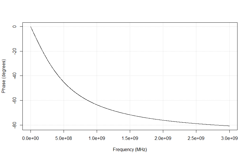
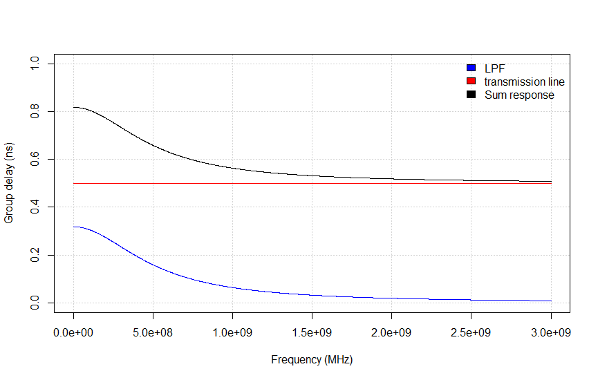
Another important use of the group delay parameter is to compensate for the phase change that is created solely by the fact that the DUT has some (electrical) length too. But most of the time we are interested in the phase change that is created by the function of the DUT and not the component that is caused by its sheer length. The phase change created by the function of the DUT can be observed as the ripple in a group delay plot, while the average group delay represents the electrical 'length' of the device. Figures 4a through 4e show the phase and group delay of a transmission line and a Low Pass Filter (LPF), as well as their combined effect when the transmission line is used as the LPF's feedline.
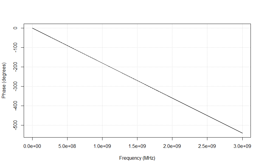
Not that in the figures below the frequency scale is linear so that a linear phase relations is represented by a straight line.
Figure 4a shows the phase response of a transmission line (for example, a coax cable) with a length (L)of 10 cm. The speed of propagation (v) in this medium is set to 2*108. The phase develops linearly with frequency. The slope of the line equals -L/v = 0.1 / 2*108 = 0.5 ns.
2.5 Return Loss and Impedance Measurements
The reflection coefficient is often expressed as the return loss (RL) in dB:
RL(dB) = - 10 Log (|Γ|2) = -20 Log (|Γ|) (4)
and, consequently
|Γ| = 10(-RL / 20) (5)
The minus sign is introduced to get a positive number that expresses a loss. The return loss is a convenient parameter to use when the value of Γ becomes small. Note, that in this conversion to return loss all phase information is lost. Therefore, the return loss parameter RL can only be used to express the mismatch of RL to Z0.
2.6 Adding VSWR to the Mix
Another much used way to indicate the amount of impedance mismatch between ZL and Z0 is the Voltage Standing Wave Ratio or VSWR for short. First, we will explain what the physical meaning of VSWR actually is and then take a look at the relations between VSWR, Return Loss (RL) and Γ.
2.6.1. The Physical Phenomenon VSWR
Again, we take a look at a wave that propagates through a transmission line which is terminated with a matched load as in Figure 4. So, there will be no energy reflected into the line. If we would observe how this wave propagates along the line, we would see that its maximum (peak) amplitude values move along the line in the direction of propagation (Animation 1). Also, at every point along the line, the amplitude of the wave is the same.
Please note that the x-axis in the animations and pictures in this paragraph represent the distance along the transmission line and not time! If you would look at some fixed point along the line you would see the amplitude at this point developing as a sinusoidal function of time. As can be observed when looking X=0.
Now we terminate the line with some impedance not equal to Z0. In this case, some energy of the wave will get reflected into the line, represented by the blue trace. This wave will interfere with the forward traveling wave (red trace) causing amplitude maxima and minima at the places along the line where the waves will add and subtract, due to their phase differences (black trace) as demonstrated in animation 2. The ratio between these maxima and minima is called the Voltage Standing Wave Ratio (figure 6).
VSWR = Vmax / Vmin (6)
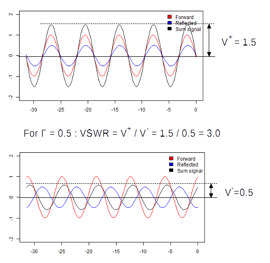
Finally, we look at the example in which the line is not terminated at all. Now, all energy is reflected, causing maxima that are double in amplitude and minima that are equals to zero (due to total cancellation). In this situation, the VSWR approaches infinity. If we would observe the direction in which these maxima and minima travel, we would discover that they are not moving (black trace). Hence the name standing wave (animation 3).
If we go back to the first case of the transmission line with a matched termination, we can now understand that the VSWR is equal to one because there is no difference in amplitude along the line.
VSWR can be measured by probing the amplitude of the wave at several points along a transmission line and, in this way, find its maximum and minimum values. From there, the ratio is easily calculated. Also, phase information can be retrieved from the position where the minima and maxima appear along the line. However, this type of measurement is, in most cases, very impractical and cumbersome. Therefore, in practice VSWR is derived by measuring the reflection coefficient which caused the VSWR phenomenon in the first place.
2.6.2. VSWR, Γ and Return Loss (RL)
From the previous section we know that VSWR is a measure of the impedance mismatch as indicated by the magnitude of the reflection coefficient Γ. In paragraph 2.3 we already learned that the Return Loss (RL) is derived from |Γ| too. So, both VSWR and Return Loss can be used to describe |Γ|. They can also be converted into each other by the following equations:
VSWR = (1 + |Γ|) / (1 - |Γ|) (7)
|Γ| = (VSWR - 1) / (VSWR + 1) (8)
and, also:
RL(dB) = -20 Log (|Γ|) = -20 Log [ (VSWR - 1) / (VSWR + 1) ] (9) using (4) and (8)
VSWR = (1 + 10(-RL / 20)) / (1 - 10(-RL / 20)) (10) using (7) and (5)
It can be helpful to look at Table 1, where we collected some common values of |Γ|, RL and VSWR to see how they are related. VSWR values are not very convenient when |Γ| gets smaller than 0.1. Return Loss expresses the complete range conveniently due to its logarithmic character. VSWR is often specified as a ratio. E.g. 1.2:1 instead of 1.2.
| |Γ| | RL (dB) | VSWR |
| 1 | 0 | Infinity:1 |
| 0.5 | 6.02 | 3.0:1 |
| 0.33 | 9.54 | 2.0:1 |
| 0.1 | 26.44 | 1.1:1 |
| 0 | Infinity | 1:1 |
| -1 | 0 | Infinity:1 |
2.7 Putting It All Together
There are a lot of applications where reflections caused by an impedance mismatch are the main concern. The mismatch can be calculated by measuring the magnitude of the reflection. That is the first class of measurements we might encounter. It uses relatively simple measurement techniques because there is no need to measure phase information as well.
The second class of reflection coefficient measurements also measure the phase change. Besides measuring the mismatch relative to Z0, we can now also calculate the impedance (both the real and imaginary parts) at the discontinuity. This technique is more complex because phase information has to be captured too.
VSWR measurements are seldom what its name suggests. Usually, VSWR is calculated from a reflection measurement instead of being measured directly.
So, it all boils down to measuring reflections. The device that is used for this task is the directional coupler, the subject of our next topic.
3. Measuring Reflections with a Directional Coupler
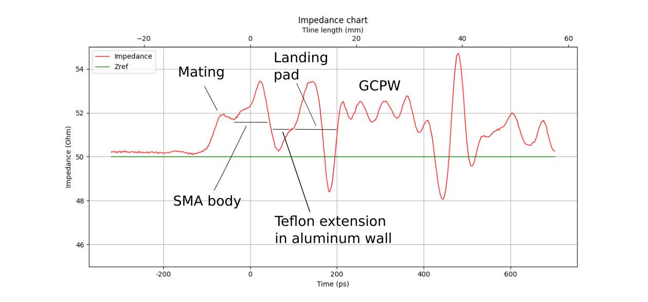
There are two fundamentally different ways to measure reflections. The first one is to measure the reflection in the time domain using a TDR (Time-Domain Reflectometer) and the second one is to measure it in the frequency domain using a VNA (Vector Network Analyzer) or SA (Spectrum Analyzer). The first method leads to results as visualized in Figure 7. The advantage of measuring in the time domain is that you can easily track the signal as it propagates through the system and, thus, separate the effect of the different discontinuities that the signal encounters during its journey.
When measuring in the frequency domain, we use the (to an RF engineer) well-known SXX-parameters and Smith Charts views to present the impedance mismatch over frequency.
Note that both views represent the same information and, indeed, the frequency domain information can be transformed to the time domain and vice versa using FFT techniques. Modern VNAs support this kind of functionality.
The advantage of a VNA or SA over TDR equipment is that they have a much lower noise floor and better dynamic range, due to their operating principle based on a narrow bandwidth sweep through the spectrum. The VNA can also add to this mix its high measurement accuracy thanks to its error correction procedures.
For these reasons, the majority of VSWR, Return Loss (RL) and SXX parameters measurements are done in the frequency domain using a VNA- or SA- based test setup.
At the heart of a reflection measurements in the frequency domain is the directional coupler. VNAs usually have them built in, while reflection measurements with an SA always use an external coupler.
3.1 What is a Directional Coupler?
From our perspective, a directional coupler is a three port device (Figure 8) which passes a test signal from Port 1 to the DUT at Port 2 (S21, Insertion Loss) and measures the signal that gets reflected at the DUT back at Port 3. Note, that the latter is attenuated by S32 (called Coupling). Therefore, the received signal at Port 3 is attenuated by an amount of (S21 + S32). When we compensate for this attenuation (by some calibration procedure) we can measure the reflected signal right away.
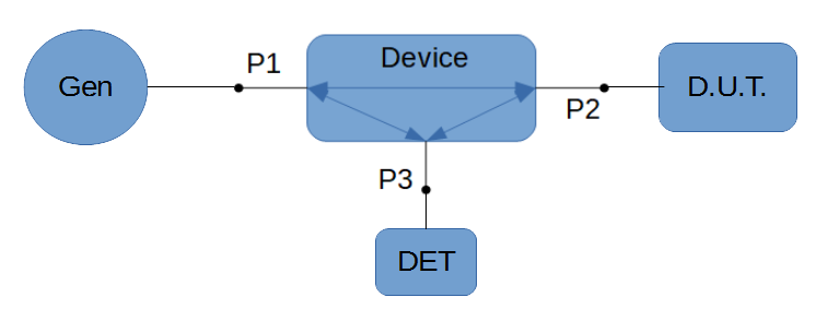
There is a catch however. In general, our three-port device will also pass the signal at Port 1 to Port 3 (S31). This can render our measurement quite useless if the signal due to S31 is strong enough to interfere with our measurement. The weaker the reflected signal, the bigger this problem will be. Also, the two signals that arrive at Port 3 add as vectors. Which will cause peaks and zeros where they are in- and out- of phase. So, we want to have a device with a S31 as close to 0 as possible.
Because we want a small S31 we call this parameters the isolation of the device. The difference between the reflected signal intensity (S21 + S32) and the interfering signal due to S31, is called the directivity D:
D = S21 + S32 - S31 (11)
The directivity has a strong effect on the accuracy of the measurement.
3.2 How to Measure Reflection with a Directional Coupler?
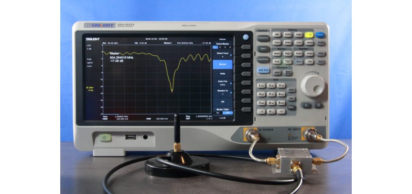
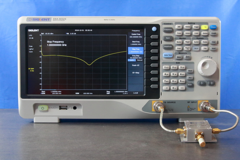
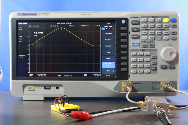
A typical return loss measurement setup is shown in Video 1. It consist of a Spectrum Analyzer (SA), a directional coupler, the DUT and cables to interconnect the components used. It may not be clearly visible from the picture, but the measurement cables are high-quality, semi-rigid cables. It is not a good idea to save on the quality of measurement cables when measuring into the GHz range. Before the setup can be used, it should be configured according to steps similar to the ones shown in Video 1. The video shows how to use a Siglent SSA 3032X spectrum analyzer while using a directional coupler.
The necessary configuration steps can be summarized as:
- Configure the SA for the frequency of interest and enable the tracking generator. The output of the tracking generator is used as the measurement sources and is connected to Port 1 of the directional coupler.
- Eliminate the effect of S21 + S32 in the SA reading. We do this by using an open termination at Port 2 so that all energy is reflected. So, what you see at the SA is just the effect of S21 + S32 alone. Now, use the normalization function of the SA so that this trace is seen as the 0dB level.
- Evaluate the directivity of the coupler to get a feel of the accuracy we can expect from this measurement setup. After the normalization step, connect a perfect 50-Ohm termination at Port 2. Now, there will be no energy reflected back. So, we only see the level created by S31 minus (S21 + S32) because that is the level at which the SA is normalized to. Put in other words, we are looking at the directivity right away. Easy! (Figure 9).
If the coupler has a high S21 + S32 (that is, a high insertion loss and low coupling) the measured signals can get quite weak. So care must be taken to keep the noise floor of the SA low. This can be achieved by using a higher tracking generator level, a pre-amplifier and lowering the Resolution Bandwidth.
3.3 Measurement Errors and How to Prevent Them
There are three phenomena that have an important influence on the accuracy of a return loss measurement with a directional coupler and an SA. We will look at all of them in succession.
3.3.1 Changes in the Plane of Reference at Port 2
From Paragraph 2.4, we learned that the shear length of a transmission line changes the impedance seen at the near-end of the line. This means that one should not create any distance between Port 2 and the DUT. A VNA compensates for this error during its calibration / error correction procedure.
Figure 10 shows what happens if the plane of reference is moved by creating some distance between the DUT and Port 2 in a typical setup which uses an SA. The effect of extra line length is related to the wave length of interest, so at high frequencies there is much less additional length needed to disturb the measurement! In the example, the frequency span is from 1MHz to 1 GHz.
3.3.2 Adherence to 50 Ohms of the Coupler's Port Itself
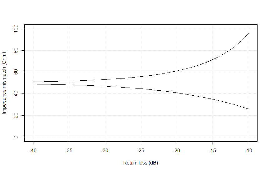
The port at which the DUT is connected should be as close to Z0 as is possible. If it is not very close to the reference impedance of 50 Ohms, we are measuring against a faulty reference impedance. For example, if Port 2 has an impedance of 60 ohms and the DUT is 50 Ohms, we will measure an impedance mismatch with in this case is a return loss of 20.8 dB.
Therefore, a good quality directional coupler must possess very well matched ports too. In Figure 11 you will find a plot of the return loss of Port 2 and its impact on impedance mismatch, based on equation (14).
RL(dB) = -20 Log (|Γ|) = -20 Log[ |ZL- Z0| / (ZL + Z0) ] (12)
We rewrite (12) as:
10(-RL / 20) = [ |ZL- Z0| / (ZL + Z0) ] (13)
ZL = Z0 (1 + 10(-RL / 20)) / (1 - 10(-RL / 20)) (14)
with Z0 = 50 Ohms.
3.3.3 Measurement Error caused by the Finite Directivity of the Coupler
Finally: a coupler with a (very) high directivity is necessary if you want to take accurate measurements on a DUT with a low return loss. In this situation, the directivity quickly becomes the limiting factor. Again, we assume the use of an SA. A VNA uses error-correction procedures to greatly enhance the accuracy and (by the way) already has its couplers built in. So, we don't pay attention to that solution in this section. Although the underlying principles of coupler directivity and the impact on accuracy are the same.
Understanding the effect of directivity on accuracy starts by realizing that in the coupler the reflected signal with a level set by (S21 + S32) and the signal from Port 1 (set by S31) both meet at Port 3 where they add up as vectors. That is the signal we observe at the SA. For the sake of this discussion, we denote the signal set by (S21 + S32 ) as the reflection signal R, and we call the signal created by S31 the isolation leakage signal L, both of which are vector quantities.

If the signal strength from R is much larger than the isolation leakage signal L, the addition of R+L will closely follow R and the SA will display an accurate measurement. When R gets lower (DUT with a better return loss) and reaches the level of L, the result of R+L will have peaks and zeros because of their phase differences. When R gets much lower than L, we will only see L at the SA and no information of R will be revealed. See Figure 12 for a visualization of the effects.
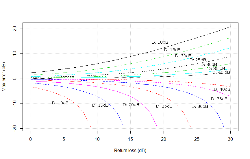
We can also plot the maximum error as a function of the return loss for a given directivity. Then we can generate a chart by plotting this error function for different values of the directivity and use it to estimate the directivity that is necessary to make a measurement for some target return loss of the DUT. With a specified maximum error.
The chart in Figure 13 is generated by calculating the maximum errors which occur when R and L are in phase (the upper half of curves) and when they are 180 degrees out of phase (the lower part of the chart). Note that the curves at the lower half of the chart run much deeper, because in this area the two vectors can actually cancel out. The chart is rendered for 7 distinct directivities, ranging from 10 to 40 dB in steps of 5 dB.
When we examine the chart, we will discover that in order to get at a reasonable accuracy the directivity of the coupler used should be quite high. For example, if we want to be able to measure a return loss of 20 dB with an accuracy of 3 dB, we already need a coupler with a directivity of approximately 35 dB. If we demand a maximum error of 1 dB, the directivity must be higher than 40 dB.
Examples of broadband directional couplers with a high directivity are:
- Gqguipment, DIRCPL-10-1-1000-A, frequency range from 1MHz to 1 Ghz with 4 dB insertion loss and 10 dB coupling.
- Gqguipment, DIRCPL-BR1-5-6000-J, frequency range from 5MHz to 6 Ghz, with 2 dB insertion loss and 15 dB coupling.
Fortunately, there also exists a whole range of return loss measurements that don't need very high accuracy. We will look at some of them in the section about Applications.
3.4 How to Evaluate a Directional Coupler?
A directional coupler should have a low insertion loss (S21), flat coupling (S32) and very high isolation (S31). There is a lot to tell about the relevant parameters of a directional coupler. The way they are designed has a great influence on their parameters. So, some insights into the design can help you to choose the right coupler for the job. There is already an article that covers a broad range of 3-port devices and its operating principles, including directional couplers.
4. Applications
Return loss measurements have many applications. In this section we will take a closer look at them.
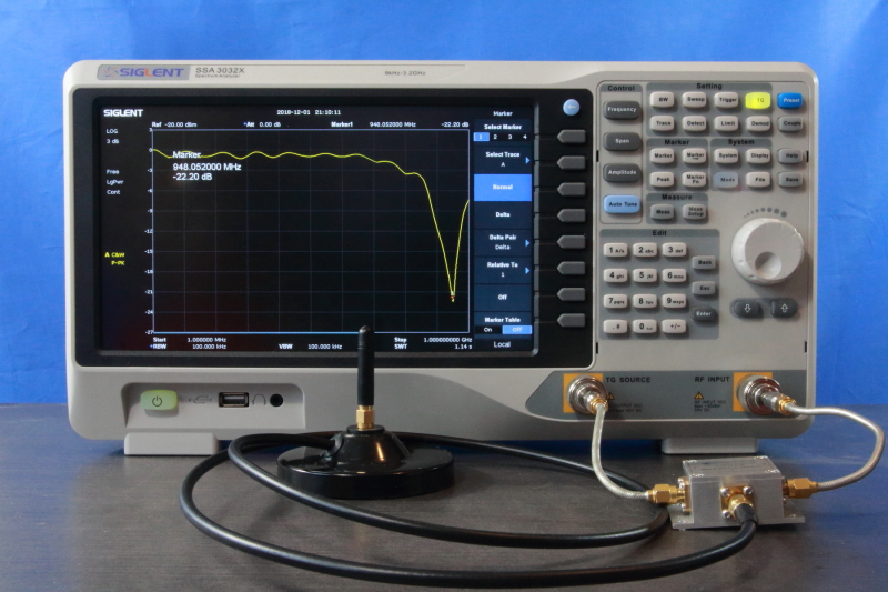
4.1. To Optimize Power Transfer
If a transmission line is not well matched with its load, it will reflect energy back into the line with less power transferred to the load as a result. An example of this situation is a power amplifier that is connected to an antenna which is not well matched to the characteristic impedance of the feed line. If the match is really bad, the amount of power reflected back into the amplifier can even destroy the amplifier circuit. Most power amplifier therefore measure the amount of reflected energy and switch off if too much energy is reflected.
To prevent such failure, the antenna’s match to the characteristic impedance is verified with a return loss measurement (Figure 14). Often, the return loss reading is expressed as a Voltage Standing Wave Ratio (VSWR). A VSWR of 1:2 or lower is, in general, considered safe. This is equivalent to a return loss of 9.54 dB. The example antenna in Figure 11 has an excellent match at 948MHz with a return loss of around 20 dB.
4.2 Minimizing Amplitude Variations
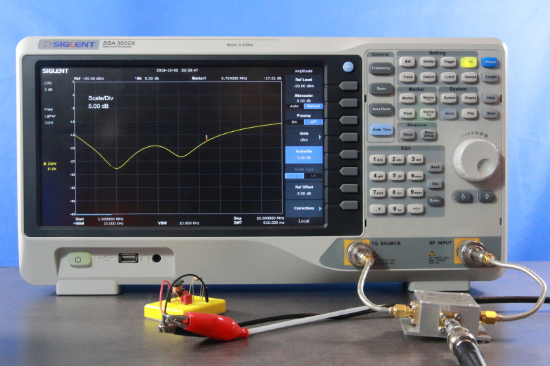
In Section 2 we learned that reflections also lead to amplitude variations in a transmission line as a function of both distance and frequency. In most applications this is not very desirable. The most fundamental way to remedy this is to create a situation in which all impedances are well matched. But this is not always possible. For example, many RF mixers have ports that are not well matched to Z0. A common solution for these kinds of problems is to add some attenuation in the line. The effect of an attenuator is that it will attenuate the incident wave and when it gets reflected the wave will be attenuated a second time. Because Return Loss (RL) is nothing more than a ratio between reflected and incident power, the RL will improve with twice the attenuation used (Figure 15).

Note that, because a long coax cable attenuates too, a VSWR measurement of an antenna at the near end of the antenna feed line will give you a better VSWR reading then when you took the measurement at the antenna port itself!
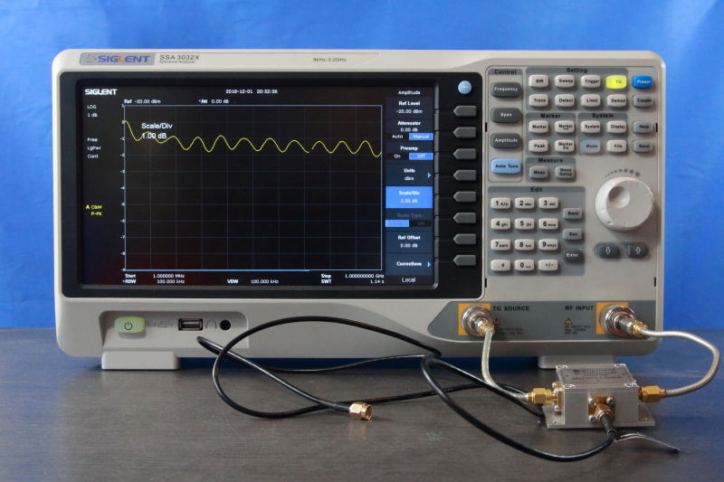
To minimize the effect of amplitude ripple, measurement cables are often connected to an SA by using attenuators to improve the RL at the SA ports. In these cases the attenuator must itself possess a very low VSWR, to not create a new source of impedance mismatch. The set-up shown in the pictures also uses two high quality 6 dB attenuators at the input and output port of the SA to improve the flatness of the frequency response of the measurement system itself.
Figure 16 demonstrates the effect of attenuation on the RL of an DUT that consist of nothing more than a not terminated coax cable.
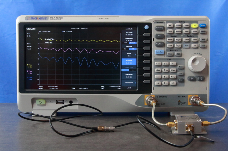
This DUT will reflect all its energy, so we expect a return loss of 0 dB. However, there is a ripple caused by the length of the cable (as explained in Section 3.3.1). If we put a 3 dB attenuator at the end of the coax (also not terminated!), RL improves by 6 dB. The same happens with an attenuator of 6 dB which creates a RL improvement of 12 dB.
4.3 Antenna Tuning
If we want to transmit RF power to air, we need an antenna. The function of the antenna is to radiate the RF energy it is fed with. It turns out that an antenna possesses a frequency dependent complex impedance at its (from our perspective) input port. Antenna tuning facilitates the power transfer from the RF amplifier to the antenna system. Note the resemblance with Paragraph 4.1.
Counter to common belief, a tuned antenna is not a necessary condition for an antenna to radiate RF energy. It merely assists in the aforementioned power transfer between antenna driver and the antenna itself.
The port of a tuned antenna will have a real impedance, meaning that the voltage across and the current flowing into the port are in phase. If the antenna is operated at a frequency in which the antenna is not resonant (or mistuned) the impedance will have a large inductive or capacitive component. Voltage and current are not in phase anymore. Energy fed to the antenna will be stored in its near field and gets returned to the antenna port. So, in this situation, the return loss of the antenna system will be very bad indeed.
All this means that we can evaluate an antenna match by measuring its impedance mismatch to Z0 By measuring the return loss of the antenna. A non-resonant antenna system in general has a large imaginary impedance component. We can see in Figure 2 (the green and red lines) that in this case all energy will be reflected as (|Γ| reaches 1. At the resonant parts of the antenna spectrum, there will be much less energy reflected (much smaller |Γ|). So, the expected return loss plot of an antenna system will be approaching 0 dB return loss with valleys (high return loss) where it is resonant (Figure 17).
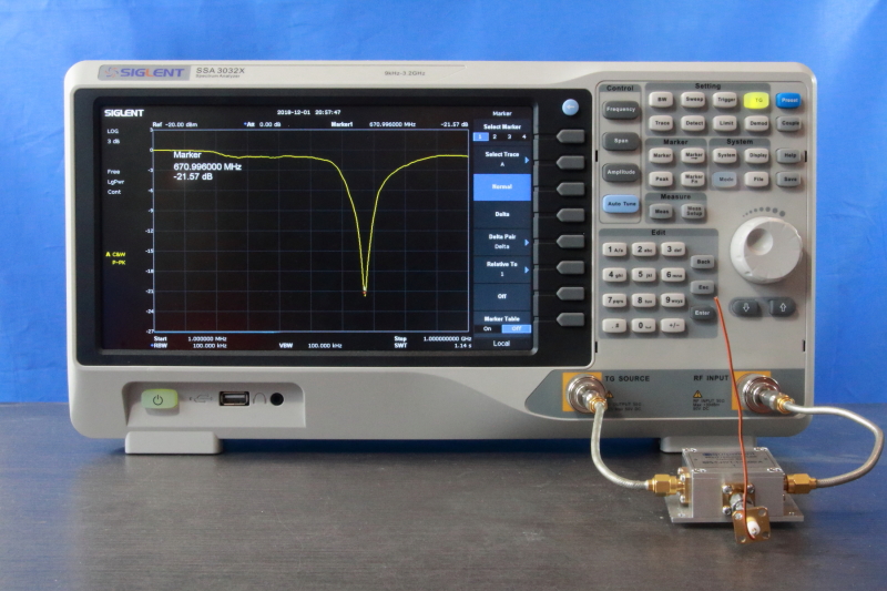
A common procedure is to tune an antenna to the desired operating frequency. A real-time return loss measurement with an SA and directional coupler assist in this procedure greatly. In this demonstration the antenna is tuned by cutting its wire to the appropriate length.
4.4 Impedance Measurement
If you want to measure impedance (instead of 'only' a mismatch to Z0) you should use a properly calibrated VNA. Due to the limitations inherent to the transformation from Γ to impedance (as visualized in Section 2) it is not possible to accurately measure impedance values without phase information.
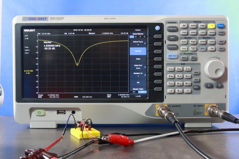
4.5 Filter Measurements
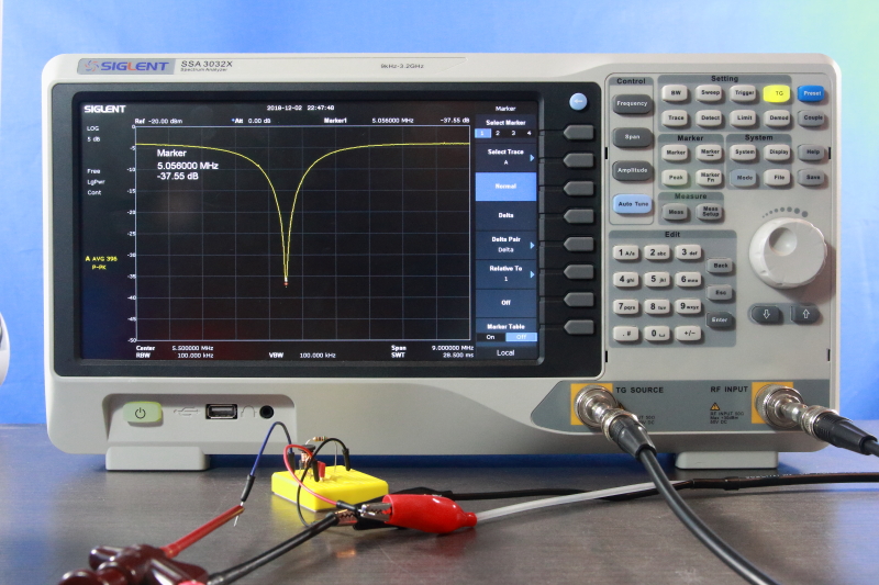
Return loss measurements can reveal some interesting properties of filters that otherwise could stay unnoticed. It is best illustrated with an example of two filters with rather similar insertion loss characteristics, but very different return loss figures. Filters with low return loss figures in their stop band(s) will reflect almost all energy back to its source. A well-known example where this could be problematic is a mixer which IF port is directly followed by some band pass filter because most mixers don't behave well when RF energy is reflected at its IF port. This situation can be solved by inserting a buffer amplifier with a matched input or by using a diplexer which has acceptable return loss figures over a broad range of operating frequencies.
In Figure 18 the same idea is shown for a notch filter. Both implementations reject frequencies around 5 MHz but differ substantially in their return loss plots.
5. Conclusion
In this article we looked at the phenomenon of return loss measurement both from a theoretical and practical viewpoint. We discovered that reflections play an important role in transmission lines and that they can tell us a lot about impedance mismatches and discontinuities. Reflections are measured with the help of a directional coupler. To make accurate measurements with an a-priori known error margin, the directivity of the coupler is one of the critical factors to consider.
However, the best way to really understand how it all works is to start experimenting by yourselves. So, get into the lab and start playing!