Transformation of time domain TDR to its frequency domain S11 (Return Loss) using FFT
In this article, we explain how to transform a time domain TDR (Time Domain Reflectometry) measurement into a frequency domain return loss graph. Since the TDR trace is in the time domain and the return loss (S11) is in the frequency domain, an FFT is used to perform the transformation. The steps are implemented using a Python script. The article concludes with some examples of different DUTs.
1. Why transform a TDR trace to return loss (S11)?
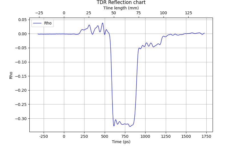
Before we answer this question, it's a good idea to summarize what the different purposes of the TDR and return loss measurements are. We start with the TDR which shows the reflection of a DUT (Device Under Test) as a function of time. Most TDRs use a step function as excitation because it is easier to implement and the reflection created matches the impedance of the DUT. It's a very intuitive way to look at a DUT because you can easily track how the impedance changes through the DUT. When the propagation speed (Vp) is known, it is also easy to convert time into distance. It is therefore a powerful technique to precisely determine the impedance at a specific location within the DUT. The resolution is limited by the step rise time and the bandwidth of the front end. Figure 1a shows an example of the reflection created by a TDR. The DUT is a Beatty, which consists of a 25 ohm trace centered in a 50 ohm microstrip (Figure 1b).
The return loss plot on the other hand, shows S11 (return loss) over frequency. Which is nothing else then the reflection coefficient (Gamma or S11) as a function of frequency, plotted in a convenient scale (dB). Of course, frequency is the domain that most of the RF engineering work takes place in, so, the return loss plot fits in naturally. And while the return loss plot also corresponds with the impedance of the DUT, the link with the physical position is not apparent anymore.
The return loss graph, on the other hand, shows S11 versus frequency. That is nothing more than the reflection coefficient (Gamma or S11) as a function of the frequency, plotted in a handy scale (dB). Of course, frequency is the domain in which most RF engineering takes place, so the return loss diagram fits naturally into this. And although the return loss also corresponds to the impedance of the DUT, the link with the physical position can no longer be found.
So why transform a TDR reflection trace into its frequency domain return loss? The first reason can be very practical: because your laboratory only has a decent TDR and no VNA. Or the bandwidth of your TDR is significantly higher than that of your VNA.
The second use case is that you want to know the return loss of your DUT, without the reflection of nearby disturbances, such as connectors or other nearby disturbances. Keep in mind that reflections interfere with each other and the end result of this interference is what you see in the return loss graph. And while it is very difficult to distinguish between these disturbances and the DUT response in the frequency domain, you can easily do this in the time domain. Using a TDR trace you can easily locate the reflection you are interested in. As long as they are sufficiently far apart from the disturbance and/or the resolution of your TDR is high enough.
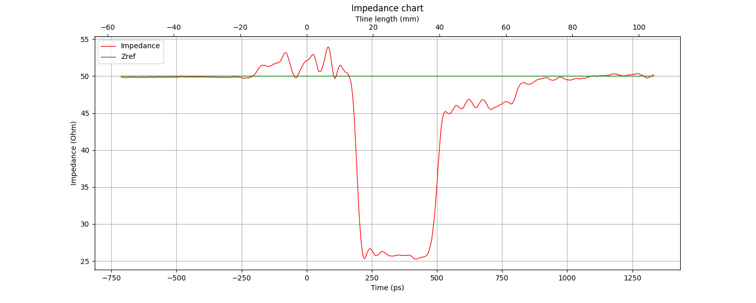
This brings us to the powerful use case of isolating the reflection of a disturbance (e.g. from a connector) and transforming it into the frequency domain to obtain the S11 parameter. This can then be used as input for a de-embedding proces to eliminate the effects of connectors on the measurements of the S-parameters of a DUT. Figure 2 shows an interesting candidate for such a procedure. It is the TDR trace of a well-matched GCPW (about 49 ohms, starting at about 70 ps) where the SMA connector (-80 ps) and the SMA landing area (between 0ps and 70 ps) create reflections that are much stronger than that of the GCPW itself.
2. The transformation process
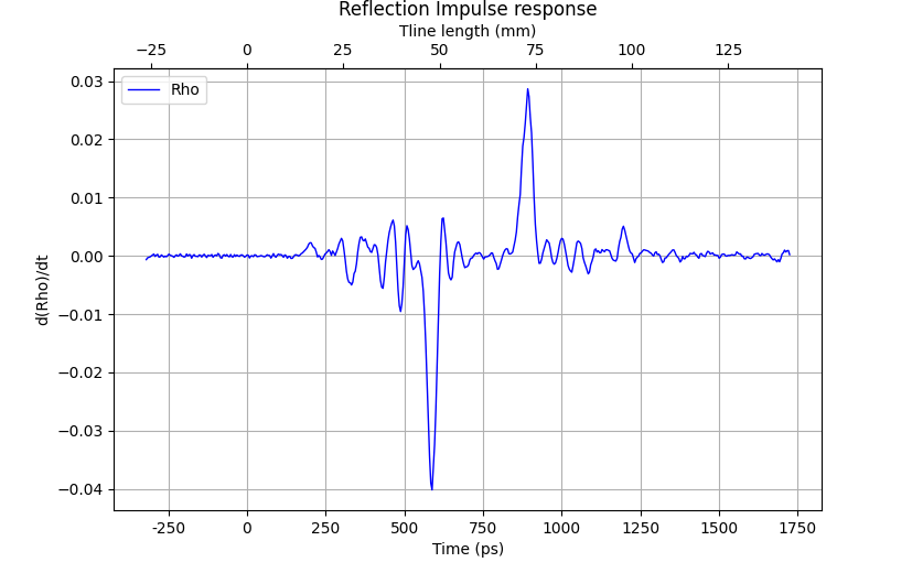
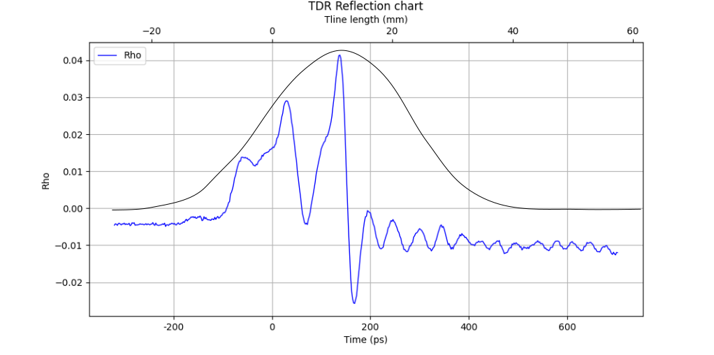
The Fourier transform and its inverse can be used to transform between the impulse response in the time domain and the frequency response in the frequency domain and vice versa. To transform a TDR time series (trace), we must use the impulse response and not the step response generated by a TDR. Therefore, the first step is to calculate the first derivative of the TDR trace, which gives us the time-domain impulse response of the reflection coefficient. Figure 3 shows the result of this operation using the same Beatty as from the previous section.
This impulse response is then transformed into the frequency domain by applying the FFT operation. This generates a frequency response with N frequency points, where N equals the number of samples of the time series (TDR trace).
Each frequency point consists of a complex number, otherwise all phase information would be lost. The spectrum also has a negative and positive frequency range. This is a result of the way each frequency point is described mathematically. Both spectra contain the same information because the positive spectrum is the complex conjugate of the negative spectrum. Long story short, you can safely discard one of the two spectra.
The magnitude and phase information can be easily retrieved from the spectrum by calculating the magnitude and phase angle for each complex frequency point. The return loss is calculated using RL = 20*Log(magnitude).
2.1 Scaling
In FFT and inverse FFT operations it is common to scale the response to maintain a certain quantity, such as power or amplitude. In our case we want to preserve the magnitude of the reflection coefficient. This is achieved by multiplying the FFT response by the sampling time. The calculation of the first derivative of the reflection coefficient does the opposite: it calculates the d(Gamma)/dt. Both operations therefore cancel each other out. Therefore, you will not find these scaling operations in the pseudocode presented in section 2.3.
2.2 The frequency dimension
The frequency axis of the return loss graph depends on several aspects such as the number of samples taken, the sampling rate and the bandwidth of the TDR measurement to name the most important ones. In this section we will explore how each affects the frequency dimension of the return loss diagram.
The most important parameters are the time steps dt (or 1/Fs) and the number of samples N. The first observation we make is that the FFT creates a spectrum of N frequency points. The time step dt defines the frequency range as (1/dt) Hz. It is easy to see that the frequency steps (the so-called bins) are distributed over the number of frequency points N. Each frequency bin therefore has a frequency resolution of 1/dt/N or Fs/N.
This relationship shows that the frequency resolution is increased by using more samples and/or increasing the time step (decreasing the sample rate). Remember that the spectrum has negative and positive frequencies, which carry the same information. Since we are throwing away half the spectrum, we only have N/2 frequency points to work with in a return loss graph. The number of relevant frequency points is also limited by the bandwidth B of the TDR measuring equipment, as there is no point in displaying frequency content outside this bandwidth. So we also have the restriction that each frequency point must satisfy fi < B.
Finally, the sampling frequency Fs is limited by the Nyquist frequency. If we assume a TDR bandwidth of B , then Fs > 2*B.
It is instructive to see how all these parameters relate to each other by putting them in a table. We used N=512 and B=20GHz.
| Time step (ps) | Fs/2 (GHz) | Frequency resolution (GHz) |
Number of points |
| 1 | 500 | 1.95 | 10 |
| 2 | 250 | 0.98 | 20 |
| 4 | 125 | 0.49 | 40 |
| 10 | 50 | 0.20 | 100 |
| 20 | 25 | 0.10 | 200 |
| 40 | 12.5 | 0.05 | 400 |
The table shows that the best results are obtained with a time step of 20 ps. The Nyquist frequency in this case is still twice the bandwidth and the FFT spectrum has 200 frequency points that fall within the bandwidth of the TDR measuring equipment. The last row in the table violates the Nyquist criterion and would also require more points than the available 256 frequency points.
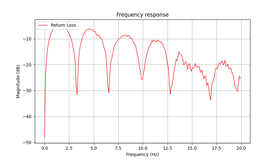
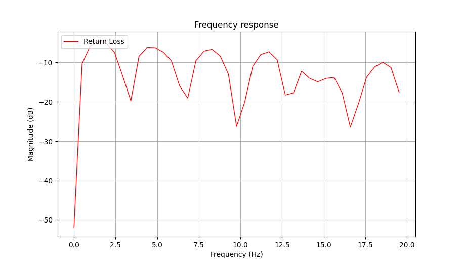
The return loss plot for a 10 ps time step is shown in Figure 4. The 4 ps version is shown in Figure 5, showing the lack of resolution and irregular pattern of peaks and valleys.
2.3 Python pseudo code
The following pseudocode summarizes the steps using Python with the NumPy library. The truncation of the spectrum to the maximum bandwidth is not shown in this code snippet.
# Trace data is in x_values
sampling_interval = np.mean(np.diff(x_values))
# First derivative
diff_gamma_values = np.gradient(gamma_values)
# FFT
fourier_data = fft(diff_gama_values)
# Get the frequencies corresponding to the FFT result
frequencies = np.fft.fftfreq(len(diff_gama_values), d=sampling_interval)
# Calculate the magnitude of the complex Fourier transform data
magnitude = np.abs(fourier_data)
# Return loss
magnitude = 20 * np.log10(magnitude)
# Plot (frequency, magnitude)
3. Some more examples
We also performed two other experiments. One with a 50 ohm transmission line because it has a relatively low reflection coefficient. And another using one of the output ports of a two-resistor splitter. It has a reflection coefficient of 0.25, which is flat over the frequency range.
3.1 A transmission line
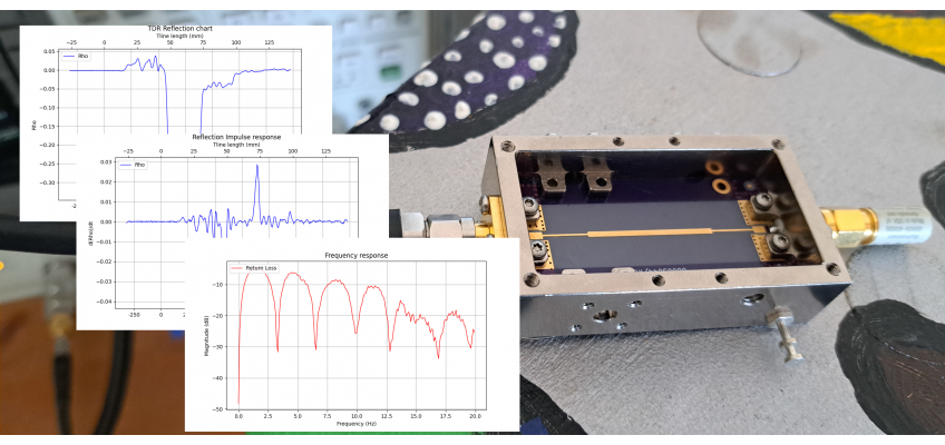
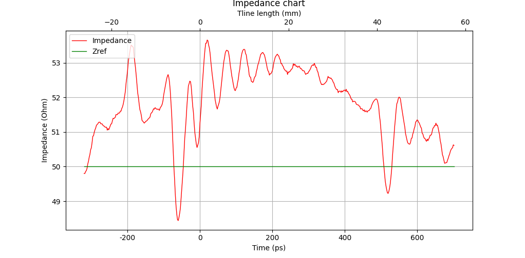
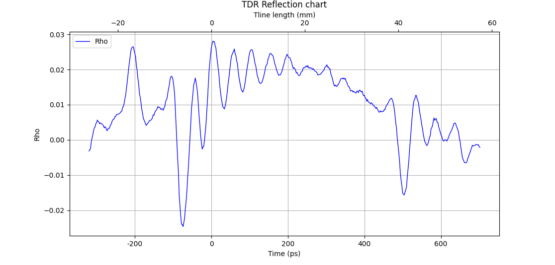
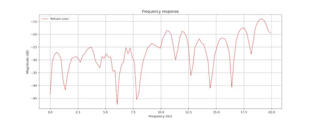
In picture 1 you can see the microstrip (GitHub PCB008003042) and a MINI-ENCL-MINI-EXT-FX used as fixture. Figure 6 and 7 show the TDR trace (impedance and reflection) and the generated return loss plot is shown in figure 8.
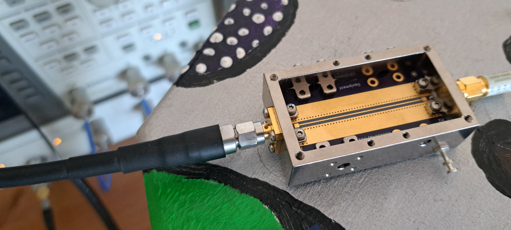
The TDR trace clearly shows that the microstrip with its 53 ohms remains within the tolerance limit of 10%. The SMA mating and connector landing areas have similar amplitude in reflections. The SMA landing area also seems to have a bit too much capacitance. This example also shows again that you can easily locate impedance discontinuities with a TDR trace.
This transmission line, with both connectors, creates a return loss graph as shown below. Up to 10 GHz the return loss is 25 dB or better, while up to 18 GHz it hovers around 20 dB. This trace has 100 frequency data points and the TDR is sampled with a time step of 10 ps.
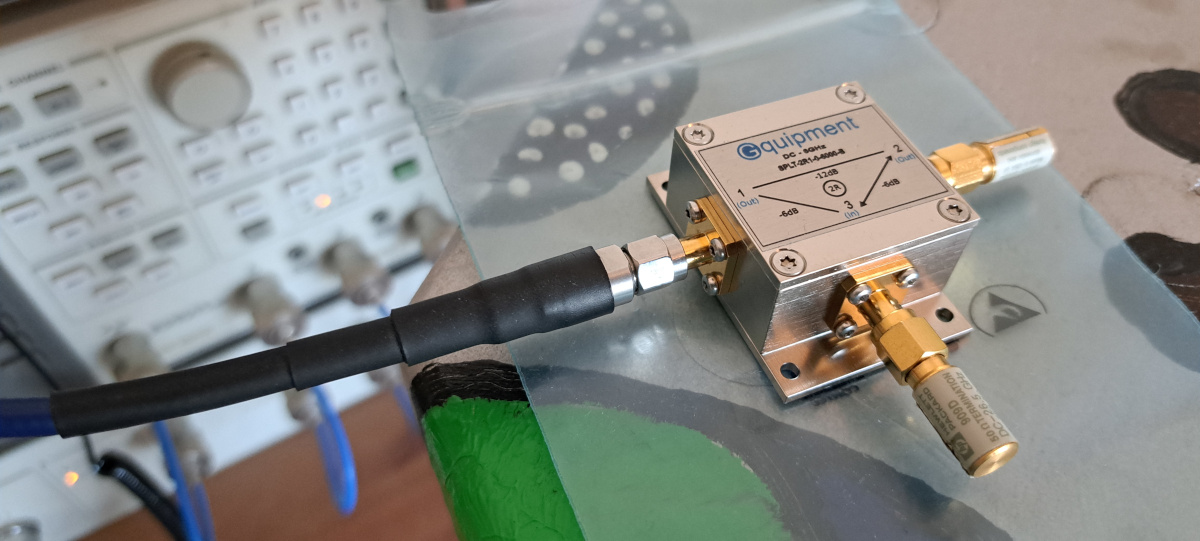
3.2 The output port of a 2R splitter
The final experiment was performed using a SPLT-2R1-0-6000-B, a power splitter that uses a two-resistor configuration. One of its features is that the output ports are not matched to 50 ohm. They exhibit an impedance of 83 ohm. This is not the place to discuss why this is the case, but here we use it as a convenient way to create a flat impedance that is not equal to 50 ohm. If you'd like to learn more about these kind of power splitters, you can check out out our overview article on power splitters and couplers.
The DTR trace clearly shows that the output port indeed has an impedance of 83 ohms. The remaining ports are terminated at 50 ohms.
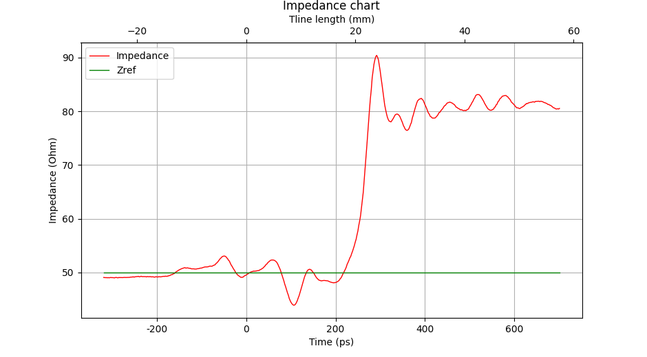
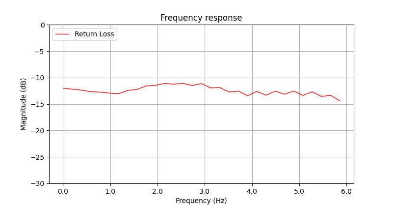
After running the Python script, we get the return loss graph as shown in Figure 10. This shows that the return loss is indeed more or less flat and centered around 12 dB, which corresponds to 83 ohms (or a reflection coefficient of 0.25). This trace was also sampled with a time step of 10 ps. The frequency axis is truncated at 6 GHz, which is the operating range of the power splitter. The chart uses 31 data points.
4. Next steps
In this article we looked at how we can use a TDR measurement to derive the return loss (S11 parameter) of a DUT. One of the issues we haven't discussed yet is that any discontinuity at the beginning and end of the time series (TDR trace) will introduce an error in the return loss. This problem can be solved by using a technique called windowing. The applied window determines which part of the trace is included in the TDR trace used for the transformation process and to what extent. You could say that in this article we used a rectangular window that started at the beginning and ended at the end of the TDR trace. It turns out that if you use a window with a shape more similar to the shape shown in Figure 11, you can minimize the errors in the return loss graph introduced by the discontinuities in the TRD trace, because they are suppressed by the applied window.
Another interesting topic is to use this windowing technique to select part of the TDR trace, in order to determine the S11 parameter of only the connectors. These can then be used as input for a de-embedding process.